The model

The model is the following discretised generalised coupled GPE:

$$ \frac{d\psi_\pm}{dt} = \left[\frac{1}{2}(Rn_\pm - \gamma) - \frac{i}{\hbar}\left(E_\pm + \alpha_\pm|\psi_\pm|^2 + \beta_\pm|\psi_\mp|^2 + K_\pm\left(n_\mp + \frac{\mathcal{P}_\mp}{W}\right) + G_\pm\left(n_\pm + \frac{\mathcal{P}_\pm}{W}\right)\right)\right]\psi_\pm - \frac{iE_{XY}}{2\hbar}\psi_\mp $$ $$ \frac{dn_\pm}{dt} = -(\Gamma + \Gamma_{s,\pm} + R|\psi_{\pm}|^2)n_\pm + \Gamma_{s,\mp}n_\mp + \mathcal{P}_{\pm} $$

This is somewhat different from the model use in a previous post in that opposite spin interactions between the polaritons are accounted for by the $\beta_\pm$ and $K_\pm$ terms. These are generally neglected, but for this specific system the behaviour we're looking for should be caused by precisely this interaction.

The procedure here is to initialize $\psi$ to small random values, run the simulation until a steady state solution is reached and find the difference in energy levels between $\psi_+$ and $\psi_-$. I do this by taking the Fourier transform of the product $\psi_+\psi_-^*$ and finding the peak of that spectrum, which gives the energy difference.

Reproduction of older results

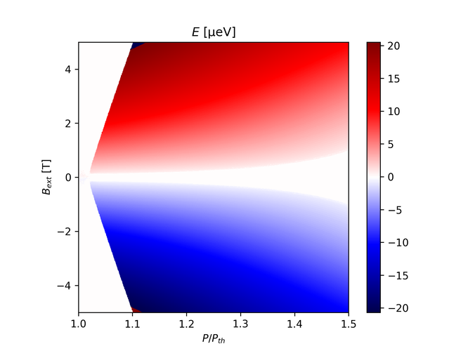
Setting $\xi=20$ and $E_{XY}=0.6$ µeV^-1 and setting $\beta$ and $K$ to 0 yields the following figure:

You'll notice there's tiny regions at the top and bottom left sides of the picture where it seems like the energy difference inverts, but this is just the FFT wrapping around.

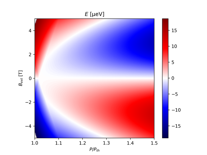
And setting $\xi=47$ and $E_{XY}=0$ µeV^-1 yields the following figure:

These are quite similar to the corresponding graphs in Sawicki et al. 2024, the difference is that the way $P_{th}$ is determined is quite simplistic. As can be seen, $P_{th}$ really depends on $B_{ext}$, but I'm using the same pump strength in each column. There's also a difference in that the energy scales seem rather off compared to the plots presented in the paper.

Anyway, this demonstrates that the more basic model is working.

Accounting for the interaction-induced magnetic field

As I mentioned in the previous post, the new model involves solving a set of non-linear equations simultaneously.

$$ B_{int} = (\alpha_+ + \beta_+)\rho_+ - (\alpha_- + \beta_-)\rho_- + (G_+ + K_+)n_+ - (G_- + K_-)n_- $$ $$ \beta_\pm = \beta_{\pm,0} \left(1 - \frac{\Delta}{B_{ext} + B_{int} \mp B_0 + ia}\right) $$ $$ K_\pm = K_{\pm,0}\left(1 - \frac{\Delta}{B_{ext} + B_{int} \mp B_0 + ia}\right) $$

Now, we can substitute for $B_{int}$ in the equations for $\beta$ and $K$ and rearrange the equations so that we have four equations in four unknowns. A set of nonlinear equation presents some problems, firstly whether a solution exists, secondly whether the solution is unique, or if it's not, whether certain solutions can be dismissed as unphysical. Assuming there exists a solution, one method to get approximate solutions for these coefficients would be to guess some values for them that are likely close to the real values, evaluate $B_{int}$, evaluate the coefficients again, etc., until the coefficients hopefully converge close to the real values. The problem is the convergence speed may not be great, and the method's may well not converge at all.

A more robust way to get approximate solutions would be to use the multidimensional Newton's method: $$ \mathbf{x}^{(k)} = \mathbf{x}^{(k-1)} - \mathbf{J}(\mathbf{x}^{(k-1)})^{-1}\mathbf{F}(\mathbf{x}^{(k-1)}) $$ Where $\mathbf{J}$ is the jacobian of $\mathbf{F}$, which is a function with a root at the desired solution. Luckily, GLSL has an inbuilt matrix inversion for matrices up to

There's also somewhat of a problem in that there's now a complex term in our coefficients. In the following I'm going to consider a somewhat simpler model that only uses the real part. The common factor in these equations is thus replaced: $$ 1 - \frac{\Delta}{B_{ext} + B_{int} \mp B_0 + ia} \rightarrow 1 - \frac{\Delta(B_{int} + d_{\pm})}{(B_{int}+d_{\pm})^2 + a^2} $$ where $d_{\pm} = B_{ext} \mp B_0$.

Results of modeling

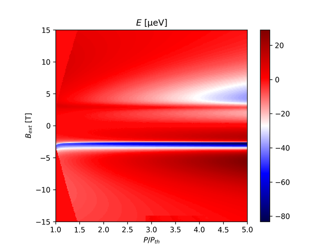
There is something odd going on with integrating this feshbach term into the simulation. The energy difference we obtain looks like this:

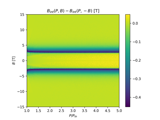
And plotting the interaction-induced magnetic field gives us the following plot:

The plots should at least be symmetric so there's certainly something wrong with the programming.