Table of Contents
Intro
The first excited states of a polariton condensate in a circular optical trap look very much like dipoles. Thus one might expect that they could be approximated decently with the first excited energy eigenstates of a 2D simple harmonic oscillator. I looked into this and found that indeed, within the optical trap, the condensate is modeled quite well by a simple harmonic oscillator. This validates a discretisation of the 2D GPE into coupled ODEs and allows a quantification of the goodness of such a discretisation.
Some of the Math and Programming
One can use the states $$ \psi_{\pm}(\mathbf{r}) = re^{-\gamma r^2 \pm i\theta} $$ as a basis for the first excited subspace of the 2D SHO Hamiltonian. Thus, one could form projection operators from this space that map it into ${\displaystyle \mathbb {C} }^2$, hence the order parameter $\Psi(\mathbf{r}, t)$ could be could be condensed into a vector of complex numbers that vary with time but are not dependent on space.
Numerically, there are a few different ways to go about such a decomposition. One could try to find various dimensions of the condensates from a snapshot of the simulation and work out the coefficients on each $\psi_\pm$ from there, either by hand or automatically somehow. In fact, when fitting a single gaussian to data a few statistical measurements are enough to specify the best fit. However, these functions do not have such a nice property, so the other option is to do least squares fitting.
There is some busywork involved in the fitting however. The entire order parameter is of course not a dipole, but several dipoles with propagating circular waves between them. This presents two possibilities: either take the entire simulation and optimise a sum of dipoles on the entire grid, or crop the grid and fit three dipoles separately. The latter option is far less computationally intensive, and is more theoretically sound. Taking a sum of all the dipoles means that the choice of coefficients on a dipole would influence the other dipoles, though only to a minuscule degree, which isn't quite in the spirit of discretising all the condensates separately. The dipole approximation also can't, and isn't intended to, capture the dynamics between condensates, and so one might get a worse approximation in the area of interest for the sake of slightly better approximating something that we don't intend to approximate anyway. It does, however, involve a bit more busywork in finding the slices needed to focus on each condensate by itself.
There is also an implementation issue one has to be careful to work around, which is that scipy's optimization tools don't support complex or 2D functions, so I had to ravel the data and gather the imaginary parts to the end of a vector.
The Results

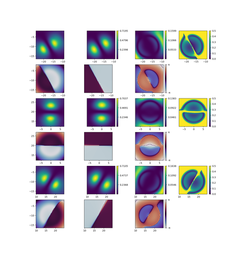
The above image (click to open it in a new tab for a better view) presents the results of least-squares fitting dipoles to the nearly exact dipoles observed in the last simulation of my post in September. Each condensate is represented by two rows. On the left is the simulated data, in the middle are values calculated with the closed form expressions, and on the right is the difference between them. The last plot in each upper row is the relative root-square error between the simulation and closed form calculation, with the color scale maxed out at 50% since relative error above that can hardly be considered a very good approximation. The upper rows colored with the Viridis colormap are the squared magnitudes of each array and the lower rows colored with the Twilight colormap are the phases of the arrays. In the area of interest, as the relative root-square error graphs show, the error is generally below 30%, and in some places where it is very high, i.e. between the poles, the actual magnitudes of both methods are very close to zero.
The fitting functions are of the form $$ f\{\mathbf{r}_0, a, b, \gamma\}(\mathbf{r}) = (a\psi_+ + b\psi_-)(\mathbf{r} - \mathbf{r}_0) $$ where the parameters in curly brackets are the fitting parameters. The centers of the dipole were initially guessed to be the same as the centers of the pumps. In fact, fitting showed the lower left dipole center was nudged 0.3 µm to the right and 0.12 µm down compared to the pump. The top dipole only had its center nudged by 0.002 µm above the pump center. The lower right dipole, however, had its center significantly displaced from the center of the pump, by almost a whole µm to the left and over 1 µm up, i.e. toward the center of the whole system.
Aside from the centers, the main fitting parameters are presented in the following table:
| Condensate | a | b | $\gamma$ |
|---|---|---|---|
| Lower left | -0.201768570 + 0.00995719196$i$ | -0.115988835 - 0.161135301$i$ | 0.0819198989 |
| Top | 0.0886651675 - 0.178488533$i$ | -0.0780398583 + 0.178428665$i$ | 0.0811440104 |
| Lower right | 0.11436693 + 0.16769492$i$ | 0.19270033 - 0.0163393$i$ | 0.08130887 |
The $a$ and $b$ coefficients are not normalised, and in fact it's important to check whether the optimization will naturally choose coefficients such that the magnitude of each condensate's state vector is approximately equal to the others. By symmetry, the condensates should be equally bright. The brightest condensate, which is the lower left one, is 1.64% brighter than the darkest condensate, which is the top one. The parameter $\gamma$ should only depend on intrinsic properties of the sample and the pump strength, which are the same for each condensate. And indeed, each condensate agrees on this parameter to within 1%.